Code
library(tidyverse)

set_theme(theme_gray(base_size = 16))While writing the Randomness Concept for the Exercism learning syllabus, there was some uncertainty about what all the various R functions do. Here, we demonstrate several them in action.
The q*() functions, to generate the quantiles, are not (yet) included.
First, we need the Tidyverse libraries and some default settings:
library(tidyverse)
set_theme(theme_gray(base_size = 16))This is the classic “bell-shaped curve”.
The dnorm() function calculates the PDF at a point: the height of the curve at that point.
Different values for standard deviation are shown. Higher values lead to wider, flatter curves.
All means default to zero.
tibble(
  "x" = seq(-4, 4, length.out = 1000),
  "SD = 0.5" = dnorm(x, sd = 0.5),
  "SD = 1" = dnorm(x, sd = 1),
  "SD = 2" = dnorm(x, sd = 2)
)  |>
  pivot_longer(
    cols = starts_with("SD = "),
    names_to = "SD",
    values_to = "value"
  ) |>
  ggplot(aes(x = x, y = value, color = SD)) +
    geom_line() +
    facet_wrap(~SD, ncol = 1) +
    theme(legend.position = "none")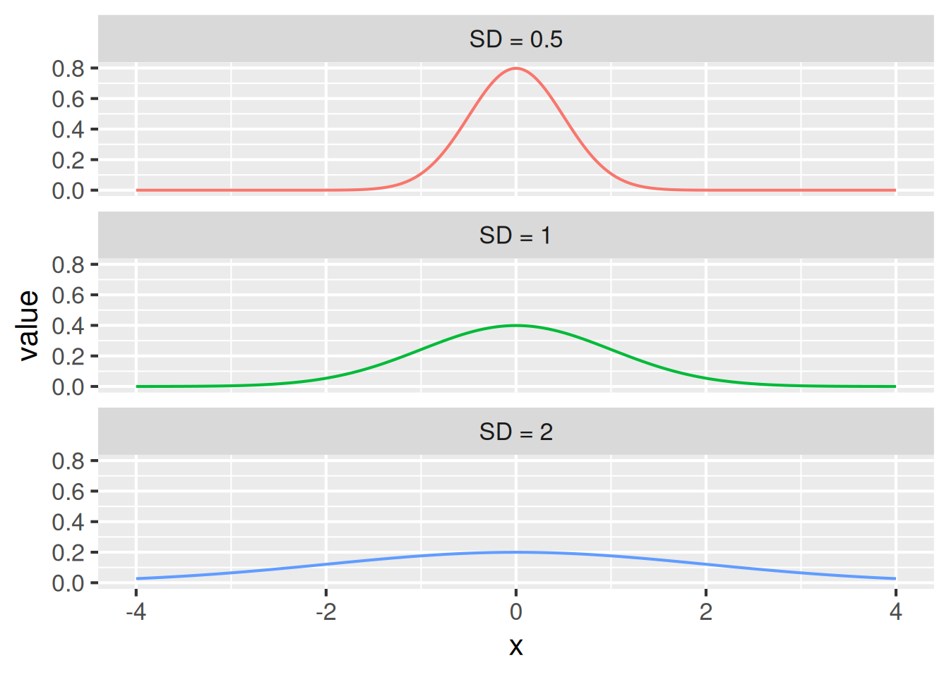
The pnorm() function calculates the CDF at a point: the integral of the curve to the left of that point.
tibble(
  "x" = seq(-4, 4, length.out = 1000),
  "SD = 0.5" = pnorm(x, sd = 0.5),
  "SD = 1" = pnorm(x, sd = 1),
  "SD = 2" = pnorm(x, sd = 2)
)  |>
  pivot_longer(
    cols = starts_with("SD = "),
    names_to = "SD",
    values_to = "value"
  ) |>
  ggplot(aes(x = x, y = value, color = SD)) +
    geom_line() +
    facet_wrap(~SD, ncol = 1) +
    theme(legend.position = "none")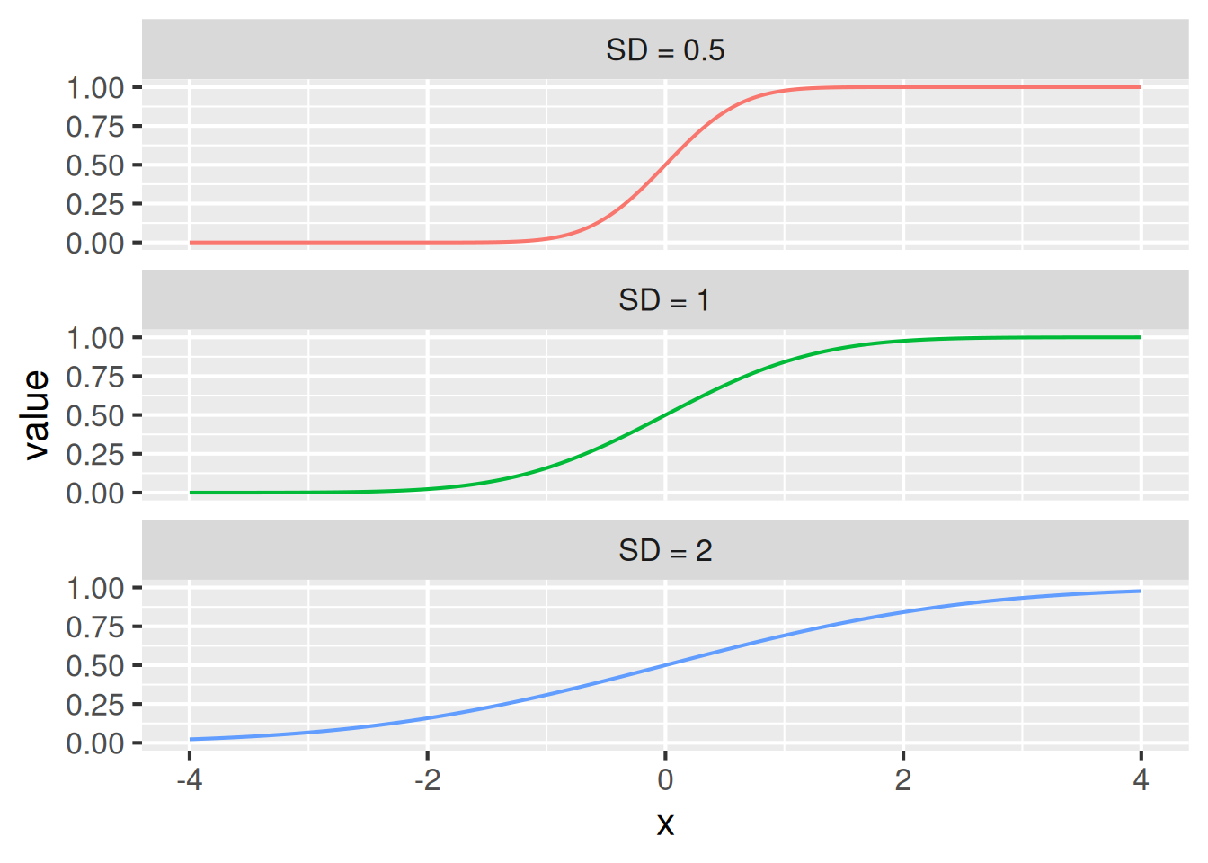
rnorm()The rnorm() function generates random values which are normally distributed.
Here, we:
y axis.n <- 10000
tibble(
"SD = 0.5" = rnorm(n, sd = 0.5),
"SD = 1" = rnorm(n, sd = 1),
"SD = 2" = rnorm(n, sd = 2)
) |>
pivot_longer(
cols = starts_with("SD = "),
names_to = "SD",
values_to = "value"
) |>
ggplot(aes(value, color = SD)) +
geom_freqpoly(binwidth = 0.05) +
xlim(-4, 4) +
facet_wrap(~SD, ncol = 1) +
theme(legend.position = "none")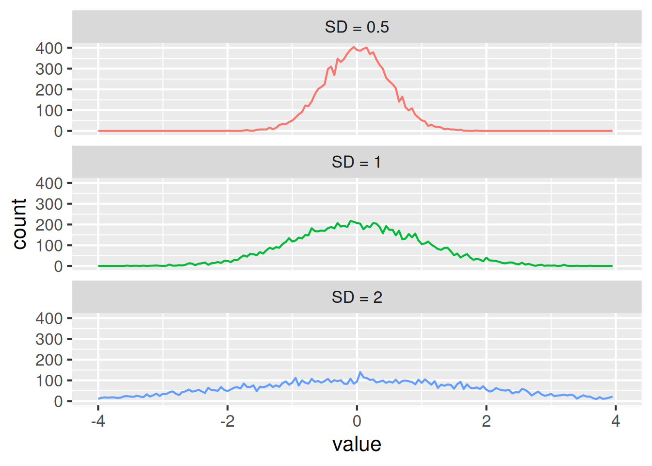
Here we use the example of 20 coin flips, counting the number that come up heads.
Three probabilities are used:
p = 0.4 for a coin biased to tails.p = 0.5 for a fair coin.p = 0.6 for a coin biased to heads.tibble(
"x" = 0:20,
"p = 0.4" = dbinom(x, size = 20, prob = 0.4),
"p = 0.5" = dbinom(x, size = 20, prob = 0.5),
"p = 0.6" = dbinom(x, size = 20, prob = 0.6)
) |>
pivot_longer(
cols = starts_with("p = "),
names_to = "p",
values_to = "value"
) |>
ggplot(aes(x = x, y = value, color = p)) +
geom_col() +
facet_wrap(~p, ncol = 1) +
theme(legend.position = "none")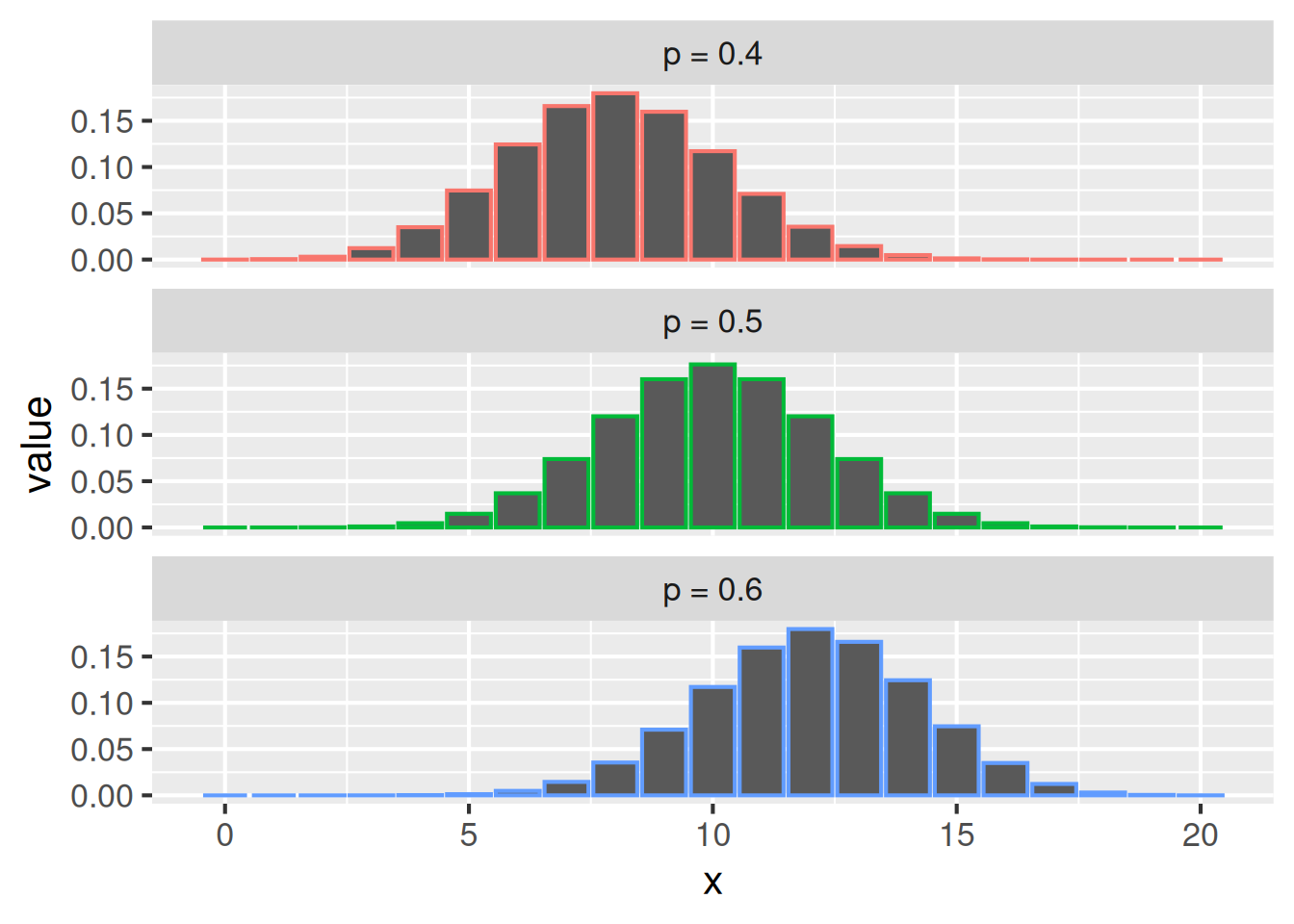
tibble(
  "x" = 0:20,
  "p = 0.4" = pbinom(x, size = 20, prob = 0.4),#| warning: false

  "p = 0.5" = pbinom(x, size = 20, prob = 0.5),
  "p = 0.6" = pbinom(x, size = 20, prob = 0.6)
)  |>
  pivot_longer(
    cols = starts_with("p = "),
    names_to = "p",
    values_to = "value"
  ) |>
  ggplot(aes(x = x, y = value, color = p)) +
  geom_col() +
  facet_wrap(~p, ncol = 1) +
  theme(legend.position = "none")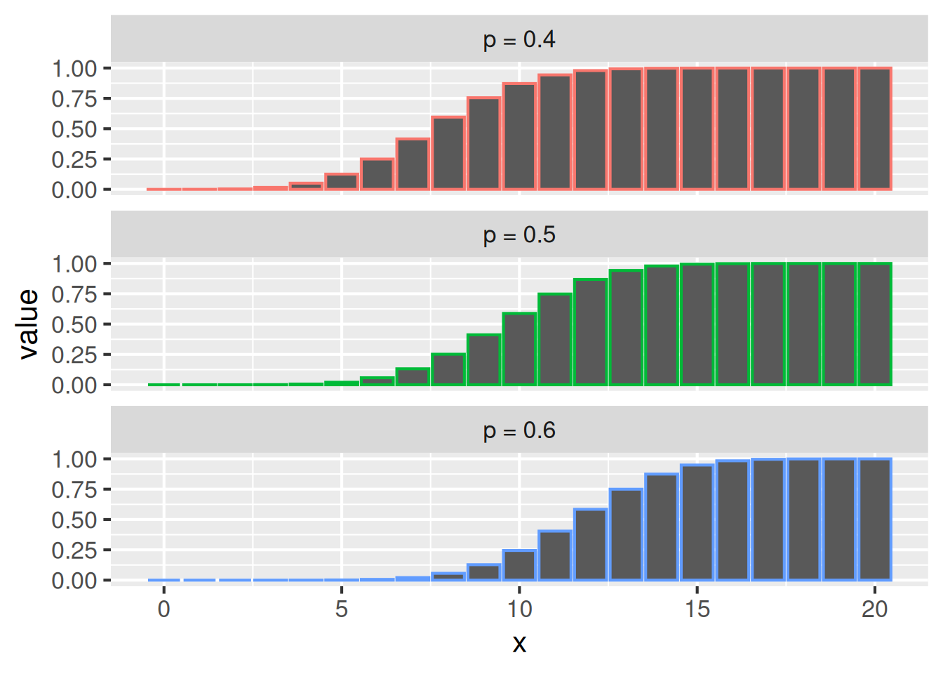
rbinom()n <- 10000
tibble(
"p = 0.4" = rbinom(n, size = 20, prob = 0.4),
"p = 0.5" = rbinom(n, size = 20, prob = 0.5),
"p = 0.6" = rbinom(n, size = 20, prob = 0.6)
) |>
pivot_longer(
cols = starts_with("p = "),
names_to = "p",
values_to = "value"
) |>
ggplot(aes(value, color = p)) +
geom_bar() +
facet_wrap(~p, ncol = 1) +
theme(legend.position = "none")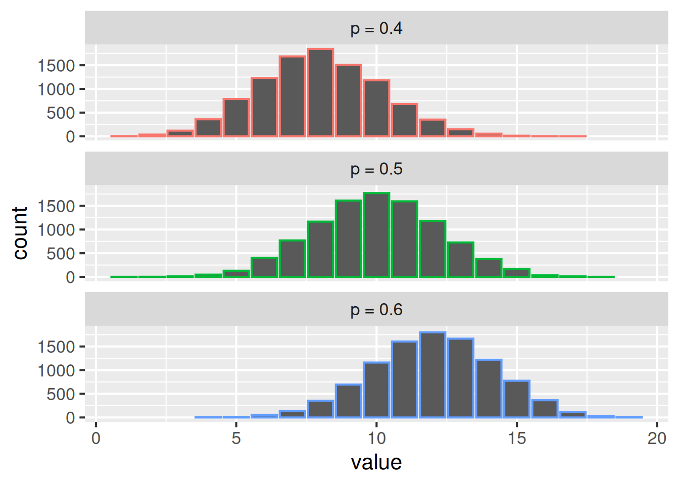
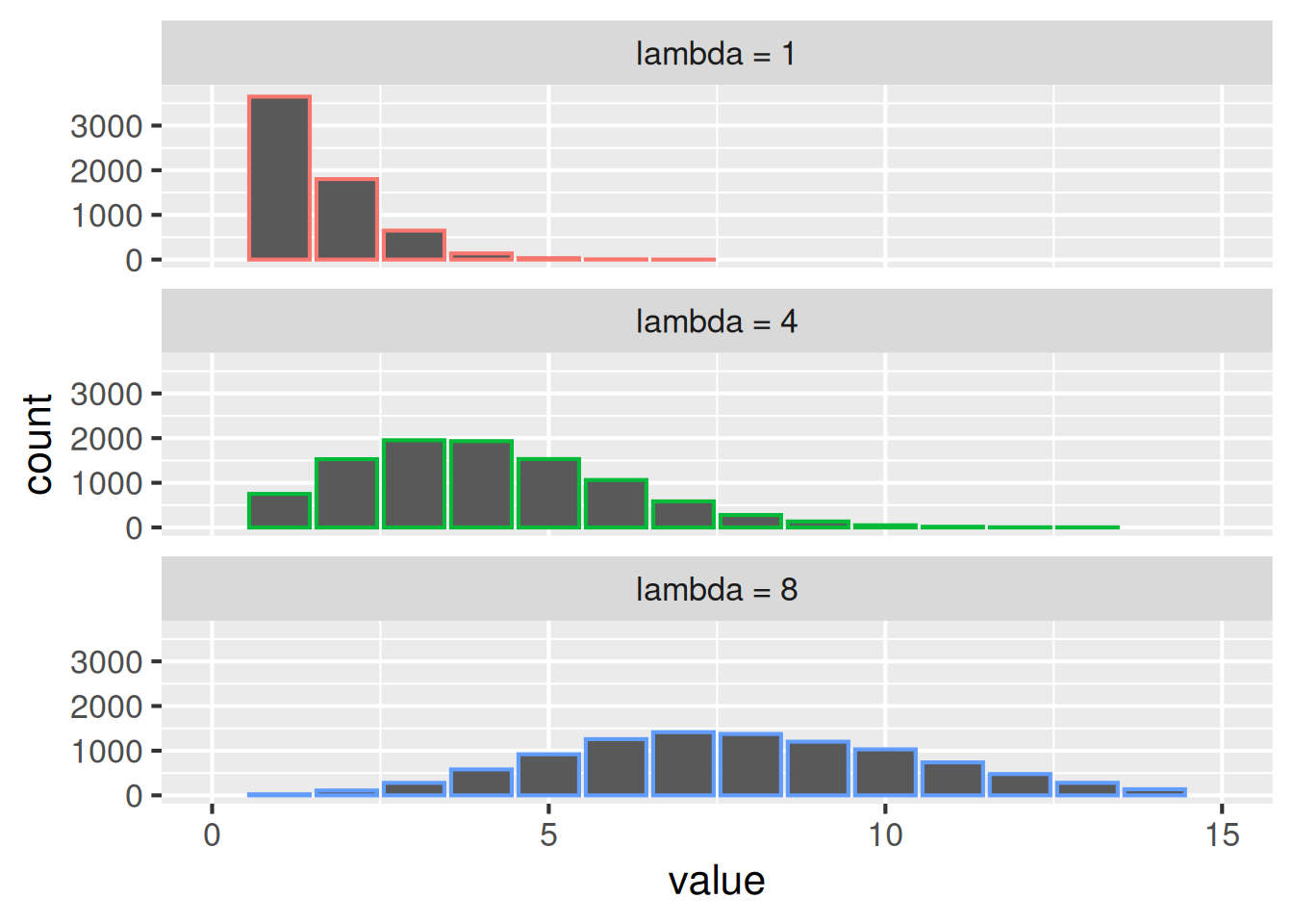
Here we use the example of how many meteorites at least 1m in diameter strike the Earth each year.
The lambda values are different assumptions for the average number. The Catalina Sky Survey discuss this and estimate such strikes happen “every few months”, so lambda = 4 is a reasonable guess.
tibble(
  "x" = 0:15,
  "lambda = 1" = dpois(x, lambda = 1),
  "lambda = 4" = dpois(x, lambda = 4),
  "lambda = 8" = dpois(x, lambda = 8)
)  |>
  pivot_longer(
    cols = starts_with("lambda = "),
    names_to = "lambda",
    values_to = "value"
  ) |>
  ggplot(aes(x = x, y = value, color = lambda)) +
    geom_col() +
    facet_wrap(~lambda, ncol = 1) +
    theme(legend.position = "none")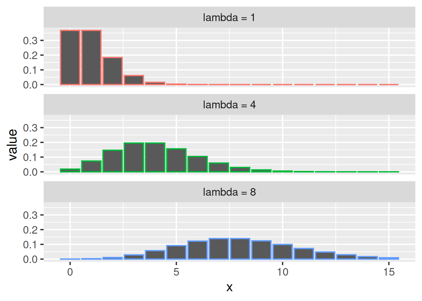
tibble(
  "x" = 0:15,
  "lambda = 1" = ppois(x, lambda = 1),
  "lambda = 4" = ppois(x, lambda = 4),
  "lambda = 8" = ppois(x, lambda = 8)
)  |>
  pivot_longer(
    cols = starts_with("lambda = "),
    names_to = "lambda",
    values_to = "value"
  ) |>
  ggplot(aes(x = x, y = value, color = lambda)) +
    geom_col() +
    facet_wrap(~lambda, ncol = 1) +
    theme(legend.position = "none")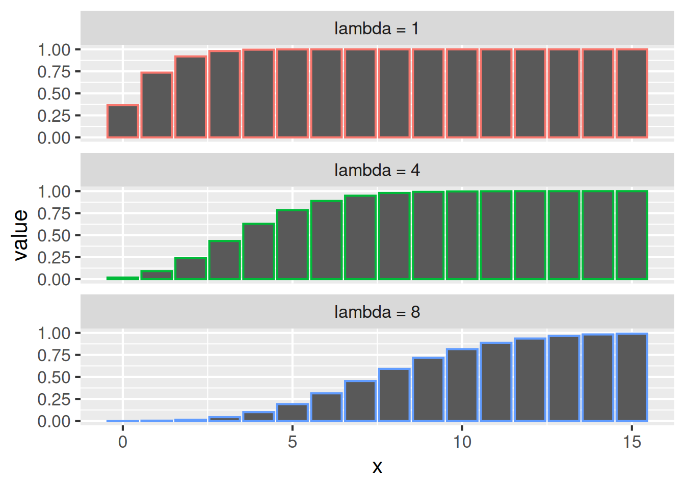
rpois()n <- 10000
tibble(
"lambda = 1" = rpois(n, lambda = 1),
"lambda = 4" = rpois(n, lambda = 4),
"lambda = 8" = rpois(n, lambda = 8)
) |>
pivot_longer(
cols = starts_with("lambda = "),
names_to = "lambda",
values_to = "value"
) |>
ggplot(aes(value, color = lambda)) +
geom_bar() +
xlim(0, 15) +
facet_wrap(~lambda, ncol = 1) +
theme(legend.position = "none")